

Introduction:
Few engineers today figure out hydraulic friction loss by hand because much of their work is done with computers. But the same basic concepts that have driven the construction of fire prevention and water-based systems for more than a hundred years are behind every computer output. It is still important to know these equations—the Hazen-Williams and Darcy-Weisbach formulas—in order to understand results, fix problems, and defend design choices. This technical note goes back over both approaches, looking at where they came from, what variables they use, how accurate they are, and how they fit into NFPA regulations. This helps modern engineers remember the basics that make hydraulic designs safe and reliable.
Hydraulic Supplement: Understanding the Friction Loss Formulas
In the age of computers, performing hydraulic calculations manually is uncommon. Design technicians and engineers rely heavily on computer-based calculations and may be less familiar, if not unfamiliar, with the formulas employed in these calculations than in previous ones. The key to mastering any topic is to first understand the fundamentals, which is why in this Tech Notes we will go over the two principal formulas used to quantify friction loss: the Hazen-Williams Formula and the Darcy-Weisbach Formula.
Hazen-Williams
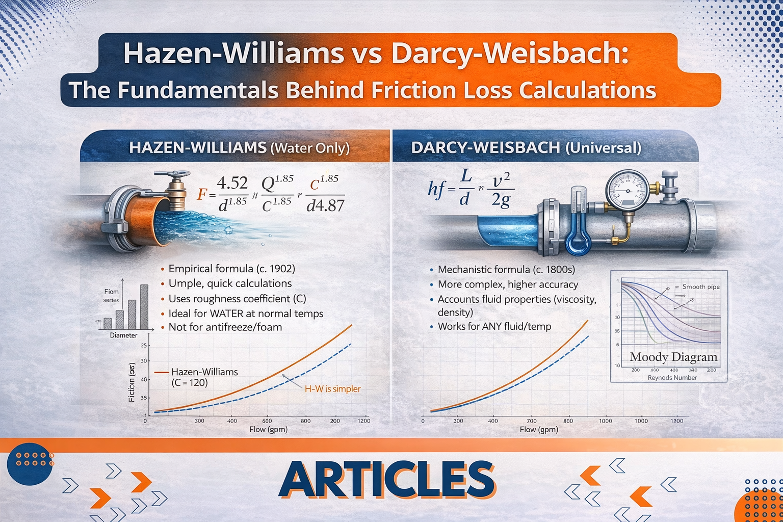
Allen Hazen and Gardner S. Williams, two American engineers, collaborated to develop the Hazen-Williams formula in the early 1900s. Their goal was to create a simple, practical method for estimating friction losses in pressurised pipes that did not rely on the sophisticated Darcy-Weisbach friction factor. Their equation was introduced about 1902, making manual calculations far easier for the design of water supply, fire sprinkler systems, and a variety of other water-based systems. While the Hazen-Williams formula provides a somewhat accurate and quick estimate of pressure loss, it is only applicable to water systems and cannot be used in systems that incorporate antifreeze or foam solutions. In sprinkler demand calculations, it gives a quick, consistent technique to anticipate loss down a single run of pipe using three inputs:
Where:
· p = Pressure loss due to friction (psi/ft)
· Q = Flow (gpm)
· d = Inside diameter (in.)
· C = Hazen–Williams roughness coefficient, C (dimensionless; higher = smoother)
What do the variables and exponents mean?
- Flow, Q (1.85): Friction increases significantly with flow. A modest increase in the needed density or the number of operational sprinklers can result in a significant increase in loss.
- Diameter, d (4.87): With the highest exponent, the diameter has the greatest impact. Upsizing a bottleneck typically reduces loss considerably, whereas shrinking accomplishes the opposite.
- Roughness, C (1.85): Smoother pipes (higher C) have less friction. C is a dimensionless empirical coefficient determined by material and condition.
- For decades, if initial estimates revealed that demand was excessive, the only variable that could be altered to make the computation work was the diameter. Upsizing pipes remains the quickest and easiest option to reduce the system’s demand pressure. However, upgrading pipelines can also be expensive. The previous two cycles of NFPA 13 have included choices for increasing the C-factor of steel pipe, at least in dry systems. NFPA 13 currently allows a C-factor of 120 for dry pipe systems that are either nitrogen-charged or have a vapour corrosion-resistant system installed. Beginning with the 2025 edition of NFPA 13, vacuum or negative pressure sprinkler systems may employ a C-factor of 120.
What Hazen-Williams is and isn’t?
- Scope and accuracy: The Hazen-Williams formula is designed for water at normal temperatures in turbulent flow over the size/velocity range typical in sprinkler systems. Within that context, it is generally adequate for design and is preferred because of its simplicity and uniformity.
- Conservatism: When compared to a comprehensive Darcy-Weisbach calculation with average commercial-steel roughness at around 60 °F, Hazen-Williams with C = 120 frequently produces similar or somewhat larger losses. Hazen-Williams is not always conservative; at very high velocities, with colder water, very rough/aged pipe, or with fluids other than water (e.g., antifreeze), Darcy-Weisbach can estimate larger losses.
- Evaluating current systems: The Hazen-Williams formula is valuable not just for calculating system demand, but also for assessing the quality of subterranean pipes. By comparing flow tests at two distinct sites along an underground line, the pressure difference can be utilised to compute the pipe’s C-factor. Low C-factor values could indicate that the pipe in question is in bad condition.
Darcy-Weisbach
The Darcy-Weisbach equation was developed in the mid-19th century, beginning with Julius Weisbach, who created the formula in its current form. Henry Darcy’s efforts helped to develop and popularise the theory, which explains the dual credit. The Moody diagram, established in 1944, provides an efficient method for determining the friction factor, which is being used today. As a result, the contemporary, generic pipe-flow loss model has become the industry standard for ensuring accuracy across fluids, temperatures, and roughness conditions.
Why Darcy–Weisbach, not Hazen–Williams, for Antifreeze?
Hazen-Williams is an empirical model for water in turbulent flow at normal temperatures that use a single smoothness coefficient (C). It does not account for variations in viscosity, temperature, or fluid density. Antifreeze solutions differ from water on all three criteria, particularly at low temperatures, hence the Hazen-Williams Formula may underestimate losses.
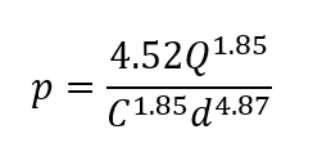
Where:
· f = Friction Factor (dimensionless)
· l = Pipe length (ft)
· p = Fluid Density (lb/ft³)
· Q = Flow (gpm)
· d = Inside pipe diameter (in)
Variable-by-Variable Breakdown
- Darcy (Moody) friction factor, f: A dimensionless factor derived from pipe roughness and flow turbulence. Derived from the Moody diagram with Reynolds number (Re = vD/v) and relative roughness (ε/D).
- Pipe length, l: The actual segment length. Length is directly proportional to friction loss; the longer the pipe, the greater the loss.
- Flow, Q: Friction loss is proportional to velocity, and pressure loss increases exponentially as flow increases. Friction losses grow with flow at a constant pipe diameter.
- The density of water is 62.4 lb/ft³, although adding antifreeze or foam solutions alters the fluid density. Fluid density increases, as does frictional pressure loss.
- Inside diameter (d): The diameter has the greatest impact on friction loss, as does the Hazen-Williams formula, because it has the highest exponent.
Where Darcy-Weisbach Makes the Biggest Difference?
- Cold conditions: As the temperature drops, viscosity rises, Re falls, f increases, and losses rise. Hazen-Williams cannot ponder on this.
- At high velocities, Darcy-Weisbach and minor-loss forecasts can outperform Hazen-Williams for water.
Comparing Graphically
The two figures below provide a comparison of friction loss using the Hazen-Williams and Darcy-Weisbach formulas. The first figure compares friction loss with water alone. As illustrated in the graph, the Hazen-Williams formula is slightly more conservative. The second image compares the two formulations after adding an antifreeze solution. In this second picture, the Darcy-Weisbach formula causes more pressure loss, but the Hazen-Williams friction loss is consistent with the water case because it does not account for changes in fluid characteristics.
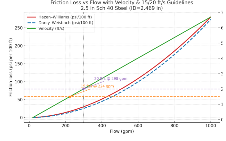
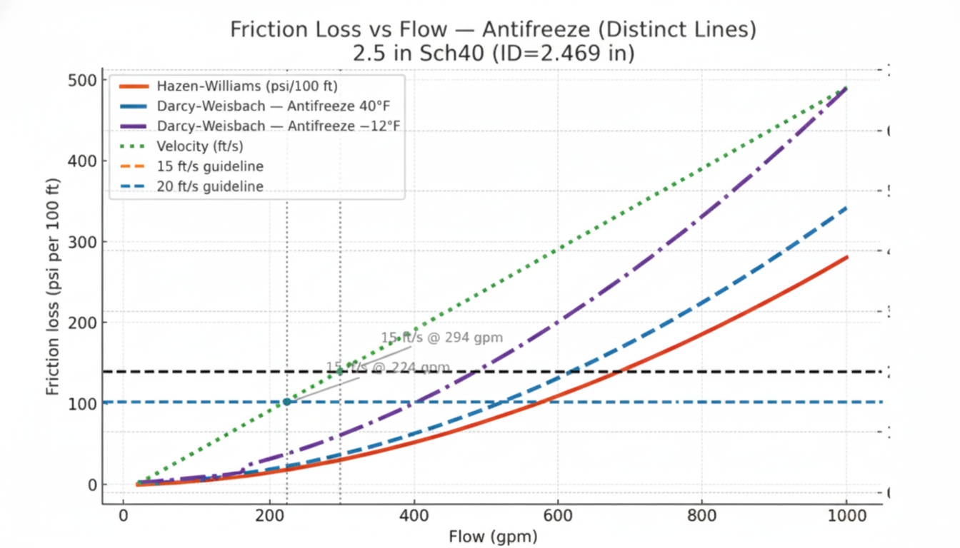
As indicated, it is critical to select the appropriate formula for the application. NFPA 13 only requires the Darcy-Weisbach formula in antifreeze systems larger than 40 gallons; however, the manufacturers of the listed antifreeze solutions need it in all antifreeze systems, regardless of size.
Conclusion
Understanding the friction-loss calculations is important because it converts a black-box printout into a sound engineering choice. When you understand what Hazen-Williams and Darcy-Weisbach assume and how variables such as diameter, flow, roughness, and fluid characteristics influence outcomes, you can identify poor inputs, select the appropriate model, and explain your decisions to reviewers. This allows you to confidently select effective fixes and troubleshoot existing systems. In short, knowing the formulas protects the safety margin, increases cost and dependability, and makes your design defendable.
Courtesy: Jeff